Testing Grid-Forming Inverters Against Realistic AI Data-Center Loads on a Power HIL Bench
A resistive load bank can pass a grid-forming inverter that real server PSUs would destabilise. How to build, verify and protect a PHIL bench that reproduces them.
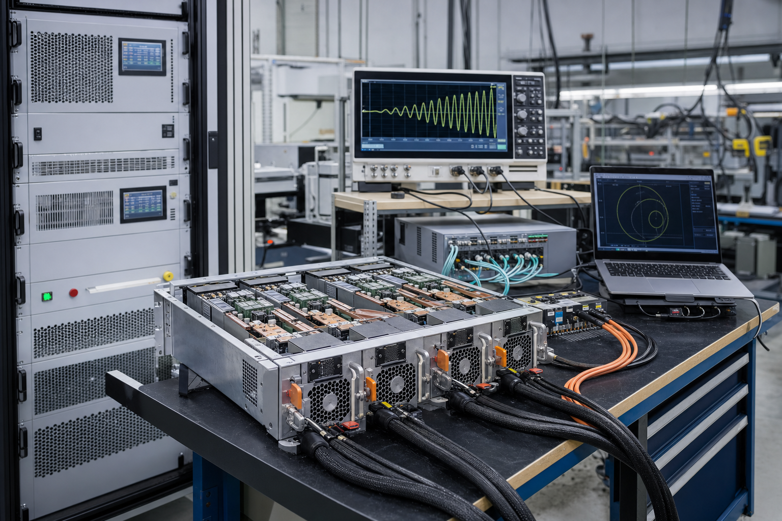
Why the load on your bench decides the result
More grid-forming (GFM) battery systems, microgrid controllers and UPS products are being sold into AI data-center projects, so more of them are being validated on power hardware-in-the-loop (PHIL) benches. The usual load on those benches is a resistive load bank, or an electronic load that tracks a power setpoint from RMS measurements. Both reproduce the MW profile of a training cluster well. Neither reproduces how the cluster behaves dynamically.
Server power supplies (PSUs) regulate their output power tightly. When the input voltage sags, they draw more current. Inside their control bandwidth that is a negative incremental impedance, , and it removes damping from the source. A resistor always has positive impedance, so a bench built around one can pass an inverter that the real load would push into oscillation. The underlying theory is covered in Why AI Data-Center Load Models Must Capture Negative Damping. This note is about the bench: how to put a realistic load on it, how to prove the load is realistic, and how to keep the hardware safe when it does go unstable.
What a resistive load hides
The figure below uses a simple per-unit model: one source with an LC resonance near 200 Hz, and the same power steps (0.10 to 0.30 pu) applied by two different load models.
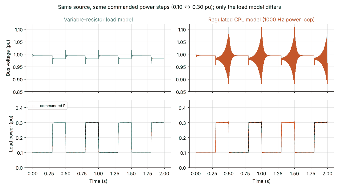
Two lessons for the bench:
- Watch voltage, not just power. In the unstable case the load still holds power close to its setpoint. A test report that only plots MW would call it a pass.
- The failure depends on the operating point. In this example the constant-power load is stable at 0.20 pu and unstable at 0.30 pu. A single test at one load level proves very little.
Three ways to load the bench
| Load option | Reproduces negative impedance? | Strengths | Limitations |
|---|---|---|---|
| Resistive bank or RMS-controlled electronic load | No | Cheap, robust, simple to control | Positive impedance; misses the interaction entirely |
| Real PSUs or PSU racks | Yes, for that PSU design | Ground truth for a specific product | Fixed design; hard to scale to MW; limited ability to sweep parameters |
| Load emulator (amplifier driven by a real-time PSU model) | Yes, if bandwidth and delay allow | Scalable, repeatable; PSU bandwidth, power and topology can be swept | Fidelity limited by amplifier bandwidth, loop delay and model accuracy |
Most serious campaigns combine the last two. A rack of real PSUs anchors the model at small scale. The emulator, validated against that rack, then represents the full cluster at its real power level.
Sizing a PSU load emulator
Bandwidth and loop delay
The emulator must reproduce both the sign and the phase of the PSU impedance across the interaction band. That band usually means the source's resonances and control bandwidths, which are typically tens of hertz to a few kilohertz. Every microsecond of loop delay adds phase lag:
With (simulator step, communication and amplifier combined), the lag is about 3.6° at 200 Hz but 18° at 1 kHz. Near −180° of load phase, 18° can turn a stable result into an unstable one or the other way round. Measure the total delay of your chain rather than taking it from data sheets, and compensate for it in the interface algorithm where you can.
Current headroom
A constant-power load draws more current as the voltage falls: . At 0.8 pu voltage it needs 1.25 times its nominal current, before any oscillation peaks are added. Size the emulator's current rating, and the bench's cabling and fusing, for the lowest voltage in the test plan plus the oscillation amplitude you intend to let develop before tripping.
Model content
At minimum, the real-time model should include the PFC current loop, the DC-link voltage loop and the output power regulation, with parameters taken from OEM data. An RMS-updated resistor running on the simulator gives you the resistive load bank's behaviour again, only at greater expense.
Verify the emulated load before you trust it
Before running any stability test, measure the input impedance of the emulated load and compare it with the target model or with the real PSU rack:
- Run the emulator at a fixed operating point, for example 50% power at nominal voltage.
- Inject a small voltage perturbation, around 1–5% of nominal, from the source side and sweep it across the band of interest, for example 10 Hz to 2 kHz.
- Record the voltage and current at the load terminals, synchronously.
- At each frequency, compute from the fundamental components.
- Check magnitude and phase. Inside the PSU bandwidth the phase should sit near −180°. If it sits near 0°, the emulator is behaving as a resistor.
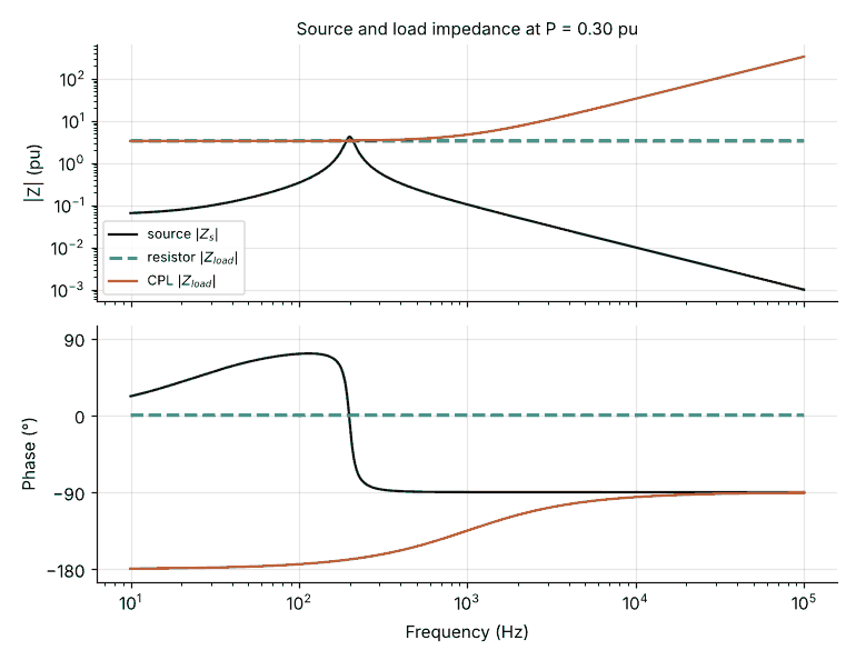
Repeat the scan at two or three power levels and at minimum voltage, because the negative impedance scales with . For three-phase AC benches, do the scan in the dq frame. That gives a 2×2 impedance matrix rather than a single curve.
A commissioning sequence that finds the edge safely
- Start with the resistive model. Confirm that the source and bench are healthy with a load that should be stable.
- Switch to the PSU model at low power. Use something like 10–20% of source rating, at nominal voltage.
- Step the power up in small increments. At each level, apply a small load step and estimate damping from the voltage ring-down, either the decay ratio of successive peaks or a fitted damping ratio.
- Plot damping against power. The trend shows where the margin will run out before you reach it, rather than after.
- Repeat at reduced voltage. Low voltage combined with high power is usually the worst case.
- Only then run the full dynamic profile, such as AI-training-style power swings, with protection armed as described below.
Interlocks: assume it will oscillate
If the test is doing its job, some configurations will go unstable. Plan for that:
- Oscillation detector on the bench, not just in the device under test (DUT). Band-pass the bus voltage around the expected interaction frequencies, compute a short-window RMS, and trip if it exceeds a threshold for more than a few cycles. Do this in the real-time simulator or the bench controller so that it does not depend on the DUT's own protection.
- Hard current limits in the emulator, set below the rating of the bench wiring, with a controlled ramp-down rather than an instantaneous open where the topology allows.
- A defined safe state. Specify what the amplifier, the DUT and any DC sources do on a trip, and test that path at low power during commissioning.
- Event capture. Arm a pre-trigger recording so that the moments before the trip are captured. That record is the useful data.
Measurement and DAQ notes
- Sample at least 20 times the highest frequency of interest. For a 2 kHz interaction band, that is 40 kS/s or more per channel. Higher rates help if you also want to see switching ripple.
- Capture voltage and current on both sides of the interface: source terminals and load terminals. Without both, you cannot separate source impedance from load impedance.
- Time-align every channel. Phase errors from unsynchronised acquisition corrupt exactly the quantity you are trying to measure.
- Log the operating point (power, voltage, model parameters) with every capture, so that results can be mapped back onto the damping-against-power plot.
FAQ
Can I scale a small rack of real PSUs up to represent the full data center? Not directly. Use the rack to validate an emulator model, then run the emulator at full power. Paralleling more PSUs adds their negative damping, but the bench quickly runs into power and cost limits.
Is a magnitude-only impedance check enough to validate the emulator? No. A resistor and a constant-power load can have identical magnitudes and opposite phases. Always check phase.
Key takeaways
- A resistive or RMS-controlled load bank can pass an inverter that real server PSUs would destabilise.
- Real PSU racks provide ground truth. An emulator validated against them provides scale and the ability to sweep parameters.
- Size the emulator for phase accuracy (loop delay) and for current at minimum voltage, not just for power.
- Verify the emulated load with an impedance scan, magnitude and phase, before running stability tests.
- Commission upward in power, track damping, and arm bench-side oscillation interlocks before running full dynamic profiles.